Representativeness Analysis: How Our Data Reflects the Real Labor Market Dynamics
This month, we will discuss the representativeness of Data@Work Research Hub data. The Data@Work Research Hub is a collection of public datasets produced by the Open Skills Project from a growing pool of public and private administrative data sources, such as job postings, resumes, profiles, etc. for the purpose of collaborative research. We have cleaned, processed, and aggregated data sources using natural language processing and machine learning algorithms. The new data includes occupations and skills across different metropolitan areas which opens a door for economists, social scientists and data scientists to study new aspects of labor market dynamics that have been difficult to analyze in the past.
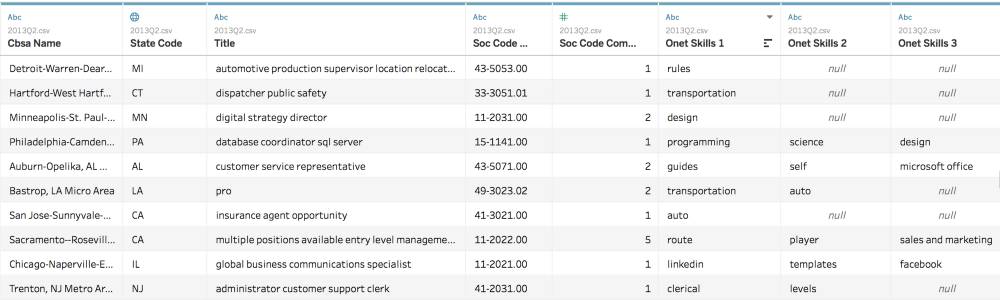 A snippet of Data@Work Research Hub data
Importance of Representativeness Analysis
Capturing the massive volumes of detailed data from job postings, non-public resumes and employment outcome data enables new analyses and implications. A good analysis depends on a good dataset, but having new data does not necessarily translate to good data. By good data, I mean representative data. Can this data represent the labor market? Is this data unbiased enough to let us build a model and draw a conclusion? In order to perform an analysis or build models among massive sampled data, we need to demonstrate the representativeness of our sampled data with confidence. Therefore, the main goal of the representativeness analysis is not only to understand our dataset from different perspectives, but also to detect bias in our dataset so that we can address it later.
Representativeness is a comparison of one’s data to the actual conditions under inspection. A representative sample is a group or set chosen from a larger statistical population that adequately replicates the larger group according to whatever characteristic or quality is under study. In our case, we want to see if our data is representative in different granular levels in order to reflect the real dynamics in labor market.
However, it is not easy to measure data representativeness. There are some major challenges in measuring the representativeness of job postings:
- There is no ground truth for the local labor demand
- Source data suffers from selection bias and duplication
- Natural Language Processing algorithms don’t catch everything
- There is potential bias in algorithms
Item #1 is tough because the real labor dynamics is like a latent variable hidden behind all available datasets. The remaining items are something we want to detect in the analysis. Having no ground truth makes representativeness analysis almost intractable, but what we can do to get a sense of what is going on in our dataset is to generate comparable statistics by occupation, geography, and time from both the Data@Work research database and relevant national labor market datasets released by the Bureau of Labor Statistics.
How did we perform representativeness analysis?
Before going any further, we should talk about how data is generated, aka sampling. The distribution of real labor market is unknown, so the only way to do the analysis is to sample data from the unknown distribution. Traditionally, researchers rely on the administration to do the survey and collect the data, such as the Occupational Employment Statistics (OES), the Job Openings and Labor Turnover Survey (JOLTS) or the Panel Study of Income Dynamics (PSID). This sampling approach is notable for the breadth and quality of data, but can be very expensive to generate. Therefore, this type of data is collected infrequently and limited in the scope of the questions that they can be used to answer. Also, not a single data set has both the geographic and temporal granularity. On the other hand, the Data@Work data sets are generated from the employment websites and state job boards data dump, which have more detailed information on job postings and it is less expensive, but this approach may have stronger noise and selection bias. Therefore, in order to understand the noise and bias in our dataset, we want to compare the Data@Work data set with two administrative data sets, the JOLTS and OES the from the Bureau of Labor Statics. The representativeness statistics we want to compare are:
- Job distribution by state (with OES)
- Occupation distribution (with OES)
- Occupation distribution correlation by state (with OES)
- Job openings time series (with JOLTS)
Analysis
Where does the data come from?
To begin with, let’s talk about the data sets. OES contains annual employment data and wage estimates for over 800 occupations, which is available for the nation, individual States, and metropolitan and non-metropolitan areas. Even though it has decent geographic granularities, it is not job vacancy data. On the other hand, JOLTS is collected from sampled establishments on a voluntary basis, including employment, job openings, hires, quits, layoffs/discharges, and separations. We are using the job openings data in JOLTS to perform the analysis. JOLTS has job vacancy information, but it is only available for the nation and 4 regions, which is not very useful in terms of the geographic granularity. The table below is a representativeness summary data overview for 2013.
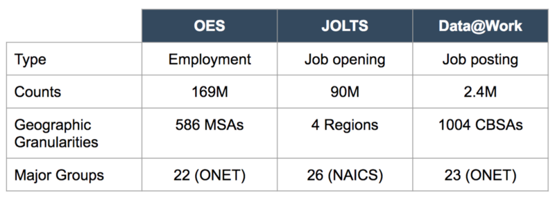
Please note that the 3 data sets are different in some sense. Even though a job opening and job posting are about job vacancy information, they are slightly different. Both the OES and Data@Work use the same occupation classification O*NET SOC codes, but the OES lacks military-related occupations. JOLTS uses the North American Industry Classification System (NAICS) to categorize their job openings. Currently, we do not have a way to convert NAICS to O*NET, which is also a reason why we cannot do much with the JOLTS data set even though it is the most related data in terms of type and time with Data@Work data.
Job distribution by state (with OES)
First, we look at the choropleth map of job distribution by state in 2013. The hue progressions represent the number of job counts aggregated in state level divided by the total job counts. The correlation is high and compatible with what we expect that California, New York, Texas and Florida have most job openings of the nation. It’s fascinating to see how correlated two data sets are.
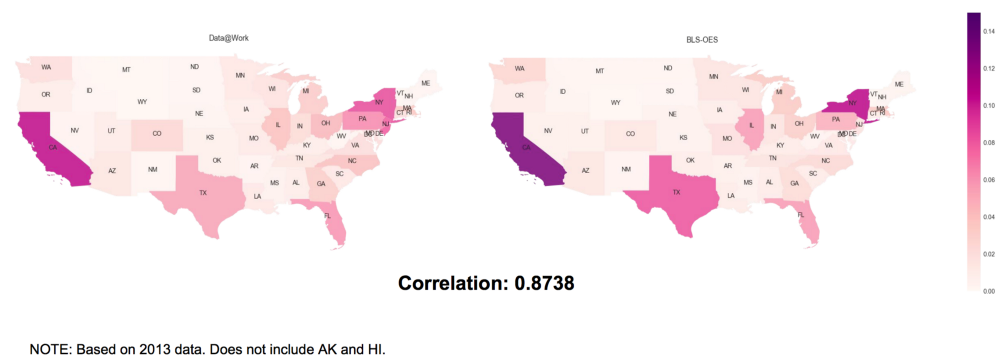 Job Distribution by State: Data@Work vs. OES
Occupation distribution (with OES)
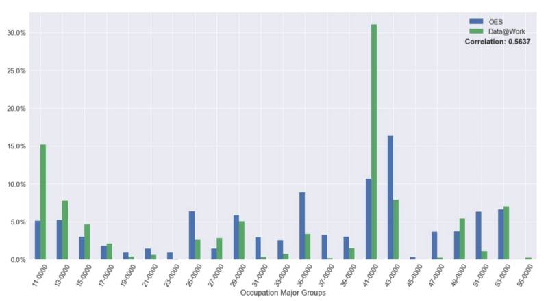
National Occupation Distribution: Data@Work vs OES. Based on 2013 data
Next, we want to analyze the difference in occupations between OES and Data@Work by looking at the percentage of job vacancy in each occupation at the national level during 2013. The lookup dictionary for the O*NET major groups is on the left. The correlation is 0.56 and it seems that Data@Work has more in Sales and Related Occupations and Management Occupations and OES has more in Food Preparation and Serving Related Occupations, Office and Administrative Support Occupations and Production Occupations. We have two possible explanations for this. First, it may be due to the selection bias in our data sources because our data sources are from one online job posting website and two state workforce boards. The other explanation is that OES is an employment data set instead of job vacancy data.
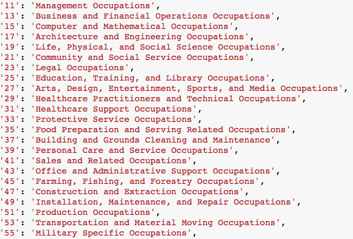 Occupation major group dictionary
Occupation distribution correlation by state (with OES)
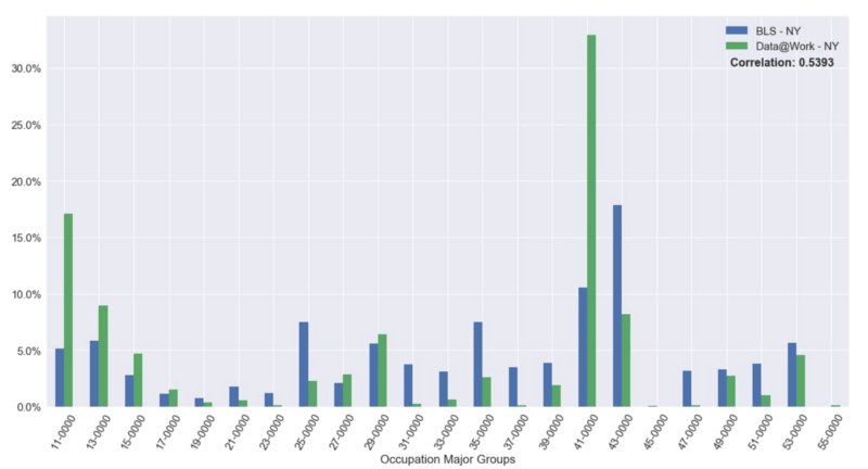 Occupation Distribution for NY: Data@Work vs. OES. Based on 2013 data
If we want to take it a step further, we can generate an occupation distribution for each state. For example, the histogram above is the occupation distribution for the state of New York and the correlation is 0.54. This is fairly similar to the occupation distribution for the whole nation since New York is one of the dominant states in terms of the job/employment numbers. We calculated the correlation of occupation distribution for every state which is shown in the choropleth map down below. The mean correlation score is 0.55 with a range of 0.44 to 0.71.
The most-correlated states are Maine and New Hampshire, and the least-correlated states are Kansas and Vermont. There are only 8 states that have correlations lower than 0.5, which are New Mexico, Rhode Island, Ohio, Kansas, Nevada, West Virginia, Wyoming, and Vermont.
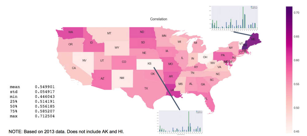 Occupation Distribution Correlation by State
Job openings time series (with JOLTS)
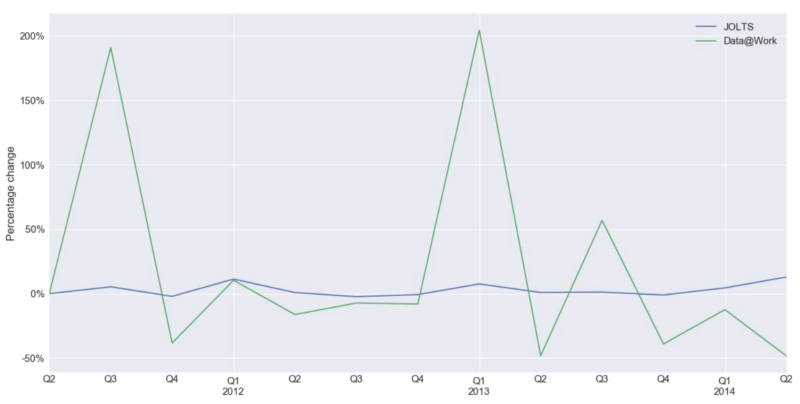
Percent Change in Data@Work Job Postings (contributed by CareerBuilder) vs. JOLTS Job Openings. Based on 2011–2014 data
The last graph is the percentage change in job openings over time. We compared the CareerBuilder data, which is one of Data@Work’s data sources, with JOLTS from 2011Q2 to 2014Q2. The reason we chose to use just a portion of the Data@Work data is because the CareerBuilder data is our most complete and continuous data source in terms of time. Other data sources are still lacking data from specific quarters, but we are looking to improve this in the future. It is interesting to see how job openings in CareerBuilder fluctuates over time and the job openings in JOLTS is steadily increasing. The percentage changes are positive most of the time, which means that job openings are increasing over time in both data sets but in different way. We are not sure why job openings in CareerBuilder peaks in 2011Q3, 2013Q1 and 2013Q3. It may be a biased behavior of one data source. Our hypothesis is that if we add more data sources, the trend may stabilize and match the results from JOLTS.
Conclusion
Based on the analyses above and assuming that the OES and JOLTS data can be used as benchmarks, then Data@Work data is partially representative. Our intention for the representativeness analysis was to give an idea of how different or similar the Data@Work data is compared with the administration data set. This helps us understand if we should do something like deduplication, resampling, or other techniques to generate better representative data for researchers. There are a couple of things that we could do to improve the representativeness analysis:
- Build a converter/classifier of NAICS to O*NET so that we can use JOLTS to its fullest extent
- Apply sampling method to data generating process such as representative sampling and stratified sampling
- Continue to add data to the Data@Work pool
- Improve deduplication
However, the true state of the local labor market is like a latent variable that we are trying to use data as a proxy to estimate what is occurring. In the meantime, we continue our efforts to improve the quality and quantity of our data. As data becomes bigger and better, there is a growing opportunity to not only revisit old questions, but also answer new questions by using these new contexts. We will have the most up-to-date representativeness analysis going forward on http://dataatwork.org/data/representativeness/ and our source codes can be found on https://github.com/workforce-data-initiative/skills-analysis.
This work is funded by the Alfred P. Sloan Foundation and the JP Morgan Chase Foundation